 BharatNotes
Part 9 of 9 of the Soils and Biogeography notes. The overview page has the quick revision and exam strategy for all nine parts.
Island Biogeography and Conservation
Why does a large island hold more species than a small one, and a near island more than a far one? This part builds the answer step by step: the species-area relationship, the equilibrium theory of MacArthur and Wilson, the experiments that tested it, and what it means for forests broken into fragments and for the design of protected areas.
Islands and the species-area relationship
An island is a patch of land with a clear edge and a barrier around it. Species must cross the sea to arrive, and once there they live in a fixed, limited space. That makes islands natural laboratories: biogeographers can count species on islands of different sizes and distances and look for rules. Island species are also vulnerable. NCERT notes that "The islands of Hawaii have many unique plants and animals that are threatened by introduced species and land development" (NCERT Class XI, chapter 14 "Biodiversity and Conservation", in Fundamentals of Physical Geography).
The first rule is simple: larger islands hold more species. MacArthur and Wilson's 1963 paper opens with two such plots: the numbers of land and freshwater bird species on islands of the Sunda group (with the Philippines and New Guinea), and on islands of the Moluccas, Melanesia, Micronesia and Polynesia, against island area (MacArthur and Wilson 1963, Evolution 17(4), figs. 1 and 2). The relationship is written as a power law:
S = cAz or, taking logarithms, log S = log c + z log A
Here S is the number of species, A the area, c a constant that depends on the group of organisms and the region (how many species fit on one unit of area), and z the exponent that sets how fast species are added as area grows. On ordinary graph paper the curve rises steeply at first and then flattens. On log-log paper it becomes a straight line whose slope is z. Durrett and Levin (1996) call this power form the most accepted species-area relationship (Durrett and Levin 1996, J. theor. Biol. 179: 119-127, p. 119). A review of 601 island data sets found that island species-area curves "are best represented by the power model and other simple models", and that the curve is "most commonly convex upwards, without an asymptote" (Triantis et al. 2012, J. Biogeography 39: 215-231): it keeps rising, ever more slowly, with no ceiling in the data.
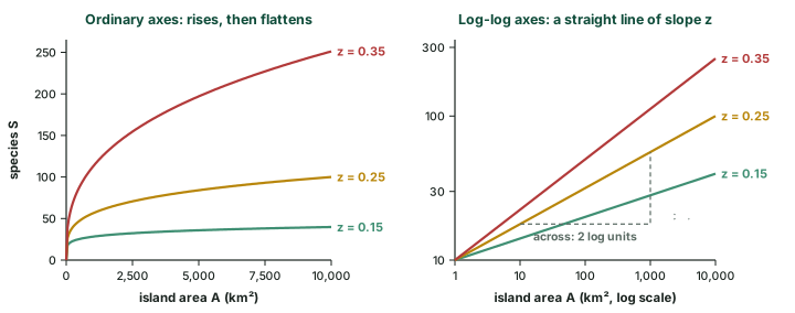
How big is z?
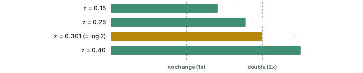
Durrett and Levin take up a question posed by Williamson (1988): "Why is the power r in general between 0.15 and 0.4?" (Durrett and Levin 1996, J. theor. Biol. 179: 119-127, p. 119; they write the exponent as r there and as z in their Table 1). Their Table 1 lists typical values, reproduced in the table below. A second analysis, by Southwood, May and Sugihara, puts it this way: "Values of z for continents are often closer to 1/3, whereas those for islands are typically slightly lower (1/8 to 1/4)" (Southwood, May and Sugihara 2006, PNAS 103). The two ranges overlap but are not the same, because they summarise different data sets. z is not a universal constant either: a meta-analysis of 794 species-area relationships found that "steeper SAR are generated at lower latitudes and by larger organisms" (Drakare et al. 2006, Ecology Letters 9: 215-227).
Typical species-area exponents z
| Group | Islands or region | z |
|---|---|---|
| Birds | Finland | 0.146 |
| Flora | Britain | 0.189 |
| Birds | Maryland | 0.213 |
| Land vertebrates | Lake Michigan Islands | 0.239 |
| Birds | East Indies | 0.280 |
| Mammals | East Indies | 0.280 |
| Ponerine ants | Melanesia | 0.300 |
| Amphibians | West Indies | 0.301 |
| Birds | East-Central Pacific | 0.303 |
| Land plants | Galapagos Islands | 0.325 |
| Carabid beetles | West Indies | 0.340 |
| Birds | Gulf of Guinea | 0.489 |
Source: Durrett and Levin 1996, Table 1 "Some typical species-area curve powers z" (Durrett and Levin 1996, J. theor. Biol. 179: 119-127), with slopes taken from MacArthur and Wilson (1967), Preston (1962), Johnson and Raven (1973), Connor and Simberloff (1978) and van der Werff (1983).
A common rule of thumb says that a tenfold increase in area doubles the number of species. It holds only when z is close to 0.3, because 10z = 2 when z = log 2 = 0.301 (computed). Across the usual range of z, a tenfold larger island holds between 1.41 and 2.51 times as many species (100.15 and 100.40, computed).
Worked example: Using the species-area power law
An island of 1,000 km² has 40 bird species. Take z = 0.30. How many species would you expect on a similar island of 10,000 km² in the same region, and on one of 100 km²? (Illustrative numbers.)
- Find c: c = S / Az = 40 / 1,0000.30 = 40 / 7.94 = 5.04.
- Island of 10,000 km²: S = 5.04 × 10,0000.30 = 5.04 × 15.85 = 79.8.
- Island of 100 km²: S = 5.04 × 1000.30 = 5.04 × 3.98 = 20.0.
- Shortcut: each tenfold step in area multiplies S by 10z = 2.00, so there is no need to find c at all.
Answer: About 80 species on the larger island and about 20 on the smaller (computed). A hundredfold range of area gives only a fourfold range of species.
Don't confuse
The species-area relationship is a pattern seen in data: bigger areas, more species. The equilibrium theory (next section) is an explanation of why islands differ in species number. Do not write that the theory is the power law.
The equilibrium theory of island biogeography
Robert H. MacArthur and Edward O. Wilson set out the theory in a 1963 paper, "An equilibrium theory of insular zoogeography" (MacArthur and Wilson 1963, Evolution 17(4)), and expanded it in their 1967 book The Theory of Island Biogeography, Princeton University Press. They began from a puzzle: remote islands have fewer species. The older explanation was time. In their summary of it, "the number of species on islands grows with time and, given enough time, remote islands will have the same number of species as comparable islands nearer to the source of colonization" (MacArthur and Wilson 1963, Evolution 17(4), p. 374). They offered an alternative: the number of species is a balance between two rates.
Two curves
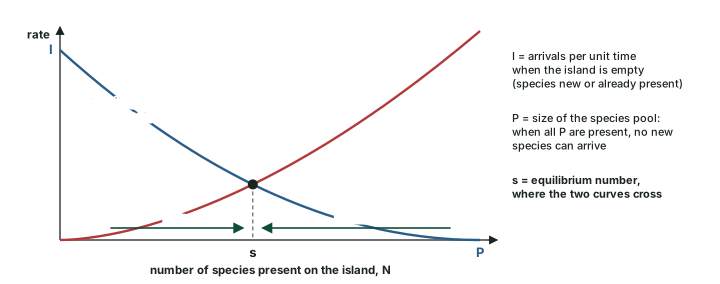
Immigration of new species. "The descending curve is the rate at which new species enter the island by colonization. This rate does indeed fall as the number of species on the islands increases, because the chance that an immigrant be a new species, not already on the island, falls" (MacArthur and Wilson 1963, Evolution 17(4), p. 374). On an empty island every arrival is new, so the curve starts high, at a value they call I. It reaches zero at P, the number of species in the "species pool" of possible immigrants: once all of them are present, no new species can arrive.
Extinction. The rising curve is the rate at which species die out on the island. With more species present there are more that can be lost, and in the authors' words "the more species there are, the rarer each is, and hence an increased number of species increases the likelihood of any given species dying out" (MacArthur and Wilson 1963, Evolution 17(4), p. 375).
Equilibrium. The curves must cross. MacArthur and Wilson call the crossing point s: "when N is greater than s, extinction exceeds immigration of new species so that N decreases, and when N is less than s, immigration of new species exceeds extinction so that N will increase" (MacArthur and Wilson 1963, Evolution 17(4), p. 377). The number settles at s. The balance is dynamic: species keep arriving and dying out, so the list of species changes even when their number stays the same. Durrett and Levin sum it up: in this theory "the number of species is a result of a dynamic equilibrium between immigration and extinction" (Durrett and Levin 1996, J. theor. Biol. 179: 119-127).
The distance effect and the area effect
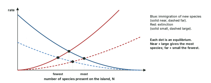
The model makes predictions without needing the exact shape of either curve (MacArthur and Wilson 1963, Evolution 17(4), p. 377):
What the equilibrium model predicts
| Change | Effect on the curves | Equilibrium | MacArthur and Wilson's words |
|---|---|---|---|
| Island farther from the source of colonisers | immigration curve lower | fewer species | "the immigration curve will be lower and hence intersect the mortality curve farther to the left" |
| Smaller species pool P | immigration curve lower | fewer species | "for the same reason" |
| Smaller island, or harsher climate | extinction curve higher | fewer species | "the mortality curve will rise and the number of species will decrease" |
Source: MacArthur and Wilson 1963, p. 377, predictions A, B and C (MacArthur and Wilson 1963, Evolution 17(4)).
Put the two effects together and four kinds of island appear: a near, large island has the most species and a far, small island the fewest. In their Fig. 2, where the archipelagos are widely scattered, "the distance effect is apparent in the greater variance"; "near" islands are those less than 500 miles from New Guinea and "far" islands those greater than 2,000 miles (MacArthur and Wilson 1963, Evolution 17(4), fig. 2).
Key idea
Species number on an island = the balance of immigration of new species (falls as the island fills; lower for far islands) and extinction (rises as the island fills; higher for small islands). Near + large = most species; far + small = fewest.
In the news: 2024
2024: a niche-based alternative. A 2024 paper in Ecology and Evolution proposes a niche-based theory of island biogeography. It describes the equilibrium theory as "a widely applied dynamic theory proposed in the 1960s", and reports that "the number of climatic niches on islands is an important predictor of the species richness of plants, herpetofauna and land birds" (Beaugrand et al. 2024, Ecology and Evolution e11540). It is a proposal, not a replacement for the equilibrium theory.
Testing the theory
Simberloff and Wilson's mangrove islands
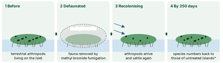
A theory about rates needs an experiment in which an island starts empty. Daniel Simberloff and E. O. Wilson supplied one. In their words, "The colonization of six small mangrove islands in Florida Bay by terrestrial arthropods was monitored at frequent intervals for 1 year after removal of the original fauna by methyl bromide fumigation" (Simberloff and Wilson 1969, Ecology 50(2): 278-296). The result: "By 250 days after defaunation, the faunas of all the islands except the most distant one" had "regained species numbers and composition similar to those of untreated islands". The slow recovery of the most distant island is the distance effect, seen in an experiment.
The species did not simply come back and stay. Observed turnover had "most values between 0.05 and 0.50 species/day"; "True turnover rates are probably much higher". They concluded that "a dynamic equilibrium number of species exists for any island" (Simberloff and Wilson 1969, Ecology 50(2): 278-296). Number restored, composition still changing: exactly the dynamic balance described above.
Krakatau
Nature ran a larger experiment. The Krakatau islands, in the Sunda Strait of Indonesia, were sterilised by the volcanic eruption of 1883 and have been recolonised since. Whittaker, Bush and Richards describe the development of their vegetation and floras since their "sterilization" in 1883, and report that "Fifty years after forest closure, the forest of the interiors remain species-poor and composed of typical early-seral species" (Whittaker, Bush and Richards 1989, Ecological Monographs 59(2): 59-123). Rebuilding a rich community is slow.
Krakatau also shows how colonists travel. "Krakatau, in Sunda Strait, is about equidistant from Java and Sumatra" (Thornton et al. 2002, Biological Journal of the Linnean Society 77(3): 275-317). The nearby island of Sebesi could have served as a stepping stone, yet many of the species that reached Krakatau are unknown on Sebesi, which suggests they arrived without it (Thornton et al. 2002).
Remember
Theory: MacArthur and Wilson, 1963 paper (Evolution), expanded in the 1967 book. Experiment: Simberloff and Wilson, 1969 report, six mangrove islands in Florida Bay, arthropods removed by methyl bromide, numbers back by 250 days except on the most distant island. Natural case: Krakatau, sterilised in 1883.
Habitat islands: when a forest becomes fragments
An island need not be surrounded by sea. A patch of forest left standing among fields, a lake among dry land, or a mountain-top habitat above a different one below are all isolated patches. When a forest is cleared piece by piece, what remains is a set of such patches, and the reasoning of the first two sections of this part applies to them. A smaller patch should hold fewer species; a patch farther from others should receive fewer colonists.
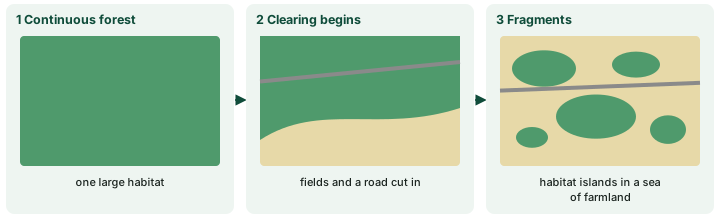
This is why the species-area relationship is used to forecast losses. A 2026 study opens with exactly that point: "The species-area relationship (SAR) has long been used to predict extirpation rates from habitat loss, but these rates depend not only on habitat area but also on the surrounding landscape and species' habitat specialization" (Bueno et al. 2026, PNAS 123(14)). The arithmetic is easy, but the second half of that sentence is the caution.
Worked example: Habitat loss and the species-area rule
A forest holds 200 species. Clearing leaves 10% of its area. Take z = 0.25. How many species does the rule predict the remnant can hold? (Illustrative numbers.)
- The constant c cancels: Snew / Sold = (Anew / Aold)z = 0.100.25 = 0.562.
- Snew = 200 × 0.562 = 112.5.
- Share expected to be lost = 1 - 0.562 = 44%.
Answer: About 112 species (computed): losing 90% of the area loses about 44% of the species in this model, not 90%. The real outcome also depends on the landscape around the remnant and on how specialised its species are (Bueno et al. 2026).
Fragment size also changes how species interact, not only how many there are. In a 2025 study, researchers "suppressed insects and fungi with biocides" in 21 rainforest fragments in the Western Ghats to measure how fragmentation affects interactions between plants and their insect herbivores and fungal pathogens; fragment size mattered (Ecological Applications 2025, e70025).
In the news: 2026
2026: habitat loss and the species-area rule. A study in PNAS (volume 123, issue 14, 2026) starts from the point made above: species-area predictions of extirpation must also account for the surrounding landscape and how specialised species are (Bueno et al. 2026, PNAS 123(14)).
In the news: July 2026
9 July 2026: IUCN Red List update. The Red List now includes 175,909 species, of which 49,505 are threatened with extinction. Five Australian marsupials, the little bettong and four mulgara species, newly recognised through taxonomic review, were confirmed Extinct (IUCN, 9 Jul 2026).
Designing reserves: the SLOSS debate
If protected areas are islands in a sea of farmland, island theory should help design them. Jared Diamond drew design rules for nature reserves from it in 1975 (Diamond 1975, Biological Conservation 7: 129-146). The application was challenged at once. Simberloff and Abele wrote: "The application of island biogeography theory to conservation practice is premature." A major conclusion of such applications, that "refuges should always consist of the largest possible single area", they argued, "can be incorrect under a variety of biologically feasible conditions" (Simberloff and Abele 1976, Science 191: 285-286).
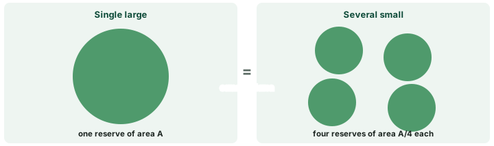
The argument became known as SLOSS: is it better to protect a single large reserve or several small ones of the same total area? A single large reserve gives the low extinction rate of a big island. Several small ones spread the risk and may together cover more kinds of habitat. Which wins depends on the species and the landscape, which is why the debate never closed.
Hypothesis, not settled fact
The rule that a single large reserve is always best is not settled. It was drawn from island theory and contested from the start (Simberloff and Abele 1976). In an answer, present SLOSS as a debate with arguments on both sides.
India's islands
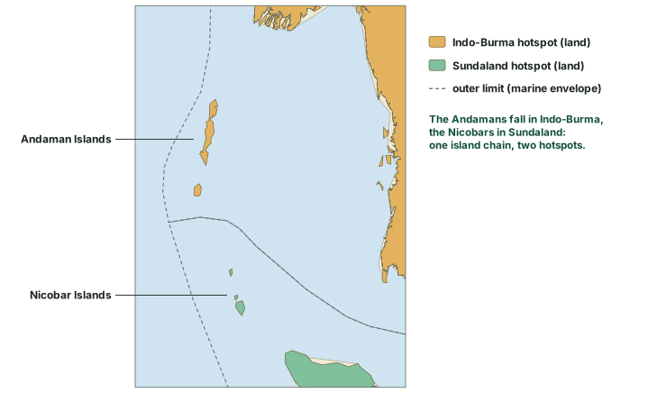
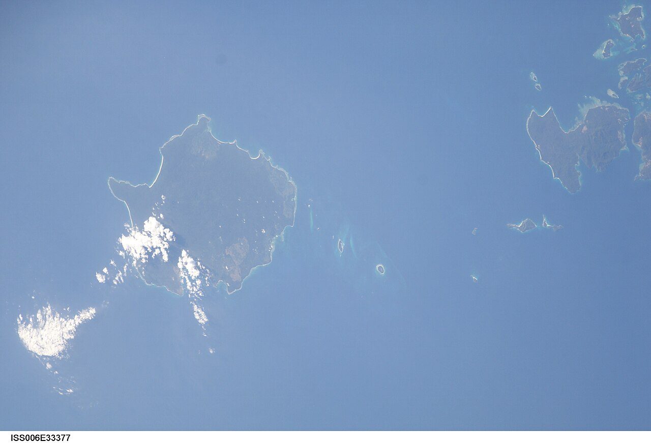
India's largest island group, the Andaman and Nicobar Islands, shows how biogeography ignores political lines. On Conservation International's hotspot map (version 2016.1), the Andaman Islands fall within the Indo-Burma hotspot and the Nicobar Islands within Sundaland. One chain of islands, under one administration, belongs to two hotspots.
The two hotspots differ in scale. Indo-Burma has about 13,500 plant species, 7,000 of them endemic; Sundaland about 25,000, with 15,000 endemic (2004 data, Mittermeier et al. 2011, Table 1.2). These are totals for each whole hotspot, not for the islands.
Island biogeography at a glance
Island biogeography at a glance
| Idea or case | Who and when | What it says or shows | Caution |
|---|---|---|---|
| Species-area relationship | pattern; power law S = cAz | bigger areas hold more species; z usually 0.15-0.4 | z varies with latitude and body size (Drakare et al. 2006) |
| Equilibrium theory | MacArthur and Wilson, 1963 paper, 1967 book | species number = balance of immigration and extinction | curve shapes are not specified by the theory |
| Simberloff and Wilson | experiment, report 1969 | defaunated islands regained species numbers by 250 days, except the most distant | arthropods on six small mangrove islands |
| Krakatau | natural case, eruption of 1883 | recolonisation of sterilised islands | interior forest still species-poor decades after closure (Whittaker et al. 1989) |
| SLOSS | Diamond 1975; Simberloff and Abele 1976 | single large or several small reserves? | unresolved; depends on species and landscape |
| Niche-based theory | Beaugrand et al. 2024 | climatic niches predict island richness | a proposal |
Compiled from the sources cited in this part: MacArthur and Wilson 1963, Evolution 17(4); Durrett and Levin 1996, J. theor. Biol. 179: 119-127; Drakare et al. 2006, Ecology Letters 9: 215-227; Simberloff and Wilson 1969, Ecology 50(2): 278-296; Whittaker, Bush and Richards 1989, Ecological Monographs 59(2): 59-123; Diamond 1975, Biological Conservation 7: 129-146; Simberloff and Abele 1976, Science 191: 285-286; Beaugrand et al. 2024, Ecology and Evolution e11540.
Summary
- Larger islands hold more species: S = cAz, a straight line of slope z on log-log axes.
- z is usually 0.15-0.4 (Durrett and Levin); islands about 1/8-1/4 (Southwood et al.). A tenfold area doubles species only when z is near 0.3.
- MacArthur and Wilson (1963, 1967): species number is a dynamic balance of immigration of new species and extinction. Far islands have lower immigration; small islands higher extinction.
- Simberloff and Wilson (1969) emptied six mangrove islands in Florida Bay; by 250 days all but the most distant had regained their species numbers, with continuing turnover.
- Krakatau, sterilised in 1883, has been recolonised since; its interior forest stayed species-poor long after forest closure.
- Forest fragments behave as habitat islands; the species-area rule forecasts losses, but the surrounding landscape matters too.
- SLOSS (single large or several small) remains a debate.
- The Andamans lie in the Indo-Burma hotspot, the Nicobars in Sundaland.
Sources
Each table and data figure names its source beneath it. The main documents are collected here, with a date where the source carries one. Figures not listed under image credits were drawn for this page from the sources stated in their source lines.
Main sources
Image credits
| Image | Credit and licence |
|---|---|
| The Andaman Islands from space, ISS Expedition 6 | Earth Science and Remote Sensing Unit, Lyndon B. Johnson Space Center, 25 February 2003 (date on its Commons page). Public domain. File page |
| All other figures | Drawn for this page from the sources given in their source lines. |